Steps to Create a Pivot Table using Data from Multiple Workbooks. Select to create the Pivot table in a new Worksheet and click on Finish.
Excel 2013 How To Create A Pivottable From Multiple Sheets Pryor Learning Solutions
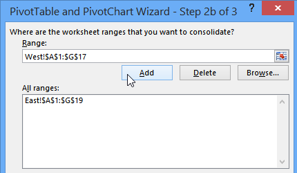
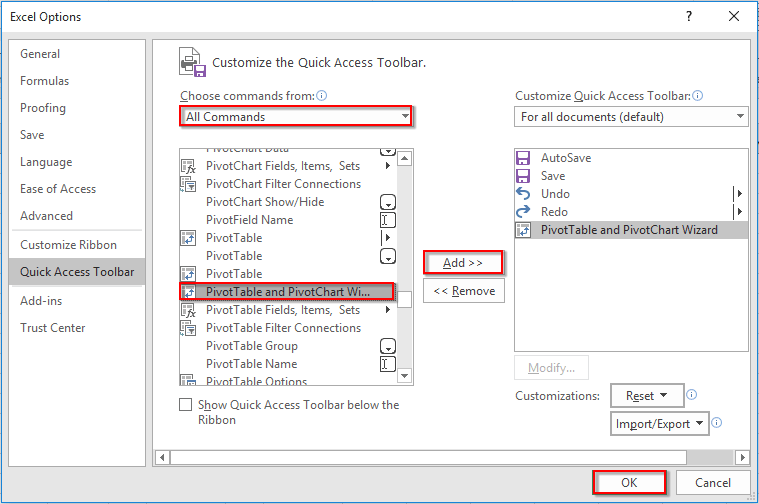
In the list select PivotTable and PivotChart Wizard click Add and then click OK.
How to do a pivot table across multiple worksheets. Those running Excel on Windows computers however can create a pivot table with data from multiple worksheets as long as the worksheets have one field in common. The steps below will walk through the process of creating a Pivot Table from Multiple Worksheets. Click on the Options drop down arrow and a fly out menu appears with the following options Options show report filter options and generate GetPivotData.
A Pivot Table is one of the best ways to summarize data. If you wish to create the pivot table in same sheet input the desired cell information from where the. But this time check the checkbox Add this data to the Data Model in order to work with multiple tables.
Its time to insert a PivotTable. 4 Select a blank cell in the newly created worksheet. One attempt to combine ranges of two sheets in the Pivot Table data range box.
Step 2 Prepare Data for the Pivot Table. In the Excel Options dialog box you need to. In the end import the data back to excel as a pivot table.
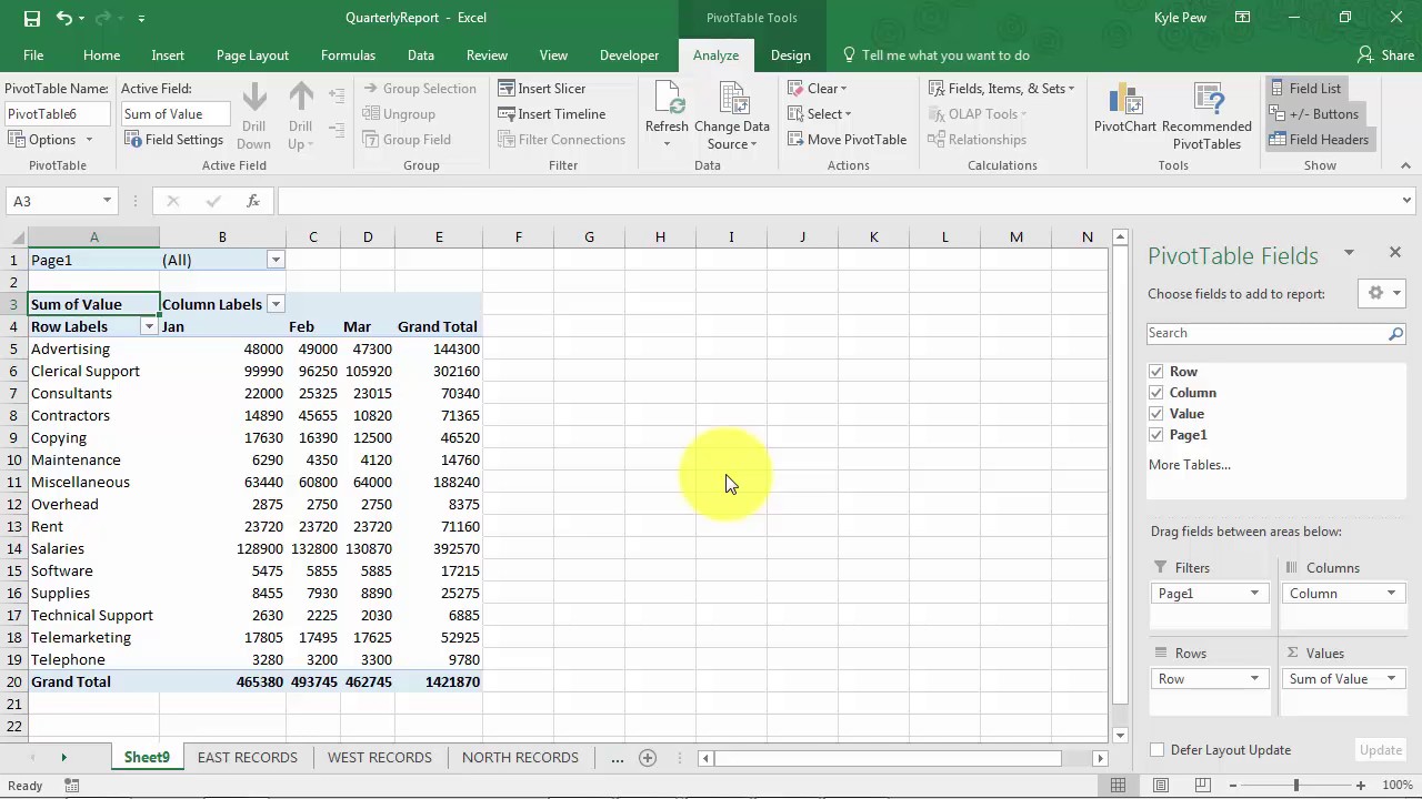
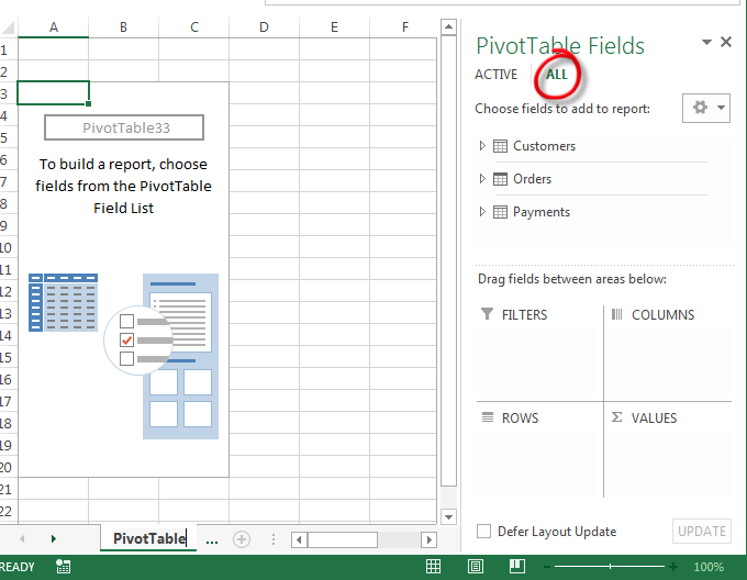
Click a blank cell that is not part of a PivotTable in the workbook. 21 Select All Commands from the Choose commands from drop-down list. Now the table that appears on the screen has the data from all the 4 sheets.
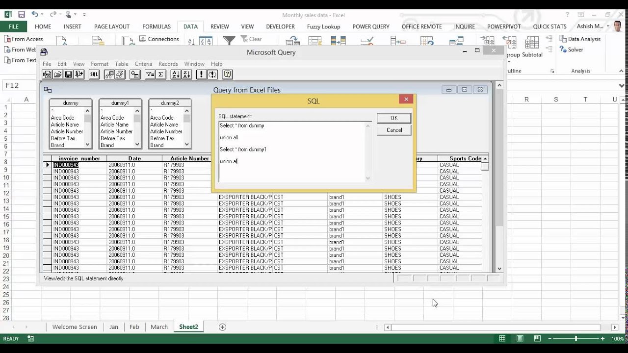
From the File Menu - click on Return Data to Microsoft Excel. All we need to do is go to File Tab and import that table into Excel. Please do as follows to combine multiple worksheets data into a pivot table.
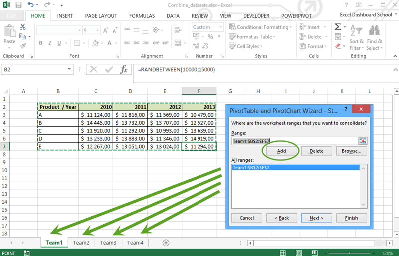
3 It is best to create a new worksheet where this Pivot Table will be located. 2 Do the same for the remaining 2 sheets containing the data you want to consolidate. To create the master pivot table from these different worksheets we need to enter into the Pivot table and Pivot Chart Wizard.
Click Customize Quick Access Toolbar More Commands as below screenshot shown. Combine multiple sheets into a pivot table. Select the Show Report filter Pages option.
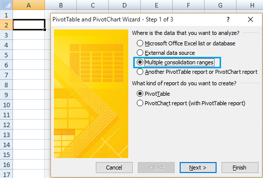
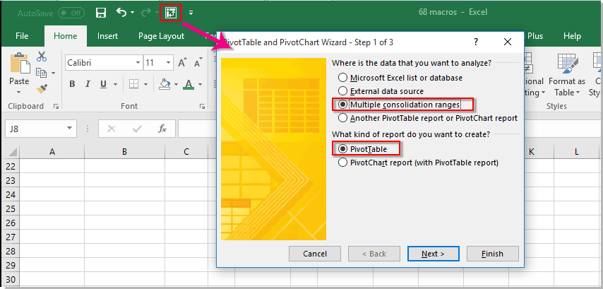
This function was disabled in earlier MS Office versions but we can access the same by the short cut keys Alt D P. On Step 1 page of the wizard click Multiple consolidation ranges and then click Next. Step 3 Insert the Pivot Table.
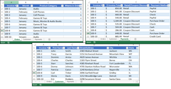
This is where we are going to Create Pivot Table using Source data from multiple worksheets. You can see that in total from all 4 sheets we have 592 records. Learn how to create a pivot table using multiple worksheets in Google Sheets.
Normally you would click OK and start working with a PivotTable. Figure 1- How to Create a Pivot Table from Multiple Workbooks. You might try combining the ranges by clicking on the symbol of four boxes beside the range of cells at the top of the Pivot table editor.
How to Create a Pivot Table from Multiple Worksheets. Select data from both the sheets and create one Page Field for each sheet. A Dialog Box will appear now and in that you will be asked whether the Pivot table should be created in a new sheet or the same sheet.
Click on the Insert tab and click on Pivot Tables. Creating a Pivot Table with Multiple Sheets. Click on any blank cell in the new Worksheet press and hold ALTD keys and hit the P key twice to fire up the PivotTable Wizard.
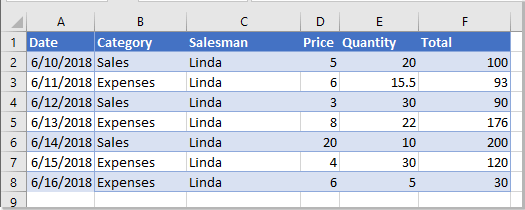
We will open a New excel sheet and insert our data. The steps below will walk through the process of creating a Pivot Table from Multiple Workbooks. Unfortunately the Pivot table editor does not allow combining ranges from different sheets of.
Step 1 Combine Files using Power Query. We can use the Power Table Wizard in Excel to create a pivot table from multiple worksheets. Pivot tables have long been a powerful tool for summarizing data and more but most of us are accustomed to using them with data from one worksheet.
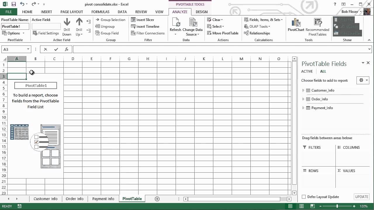
We can use the Power Pivot Add-In in Excel to create a pivot table from multiple workbooks. Confirm that the My Table has headers box is checked click OK. Clicking into the pivot activates the PivotTable Tools ribbon selecting the Options tab gives the following menu options.
5 Press Alt D and then press P. This tutorial covers cases with matching or not matching columns as well as dy. Label the Page field appropriately.
It is good to use a new sheet option in. Under Choose commands from select All Commands. Click the first Table and navigate to Insert Table PivotTable.
Setting up the Data. Here we will use multiple consolidation ranges as the source of our Pivot Table.
Consolidate Multiple Worksheets Into Excel Pivot Tables
Create An Excel Pivottable Based On Multiple Worksheets Youtube

How To Create A Pivot Table From Multiple Worksheets Step By Step Guide
Create A Pivottable In Excel Using Multiple Worksheets By Chris Menard Youtube
Create A Pivot Table From Multiple Worksheets Of A Workbook Youtube
How To Create An Excel Pivot Table From Multiple Sheets Contextures Blog
134 How To Make Pivot Table From Multiple Worksheets


How To Create A Pivot Table From Multiple Worksheets Using Microsoft Excel 2016 Basic Excel Tutorial
Excel 2013 How To Create A Pivottable From Multiple Sheets Pryor Learning Solutions
Advanced Pivottables Combining Data From Multiple Sheets

Best Excel Tutorial Create Pivot Table From Multiple Sheets
How To Create Pivot Table From Multiple Worksheets
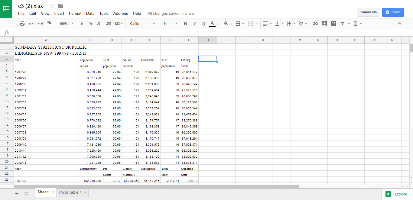
How To Work With Pivot Tables In Google Sheets
How To Combine Multiple Sheets Into A Pivot Table In Excel
134 How To Make Pivot Table From Multiple Worksheets


Advanced Pivottables Combining Data From Multiple Sheets

Best Excel Tutorial Create Pivot Table From Multiple Sheets
How To Combine Multiple Sheets Into A Pivot Table In Excel
How To Combine Multiple Sheets Into A Pivot Table In Excel


0 comments